Mathematics / Film

Revisiting the First Blackboard Problem in Good Will Hunting

What the film’s first problem actually shows, how its four tasks are connected, and where the mathematics leads.

Published 28 July 2026 Approximately 30 minutes

The scene is often remembered as a single quite impossible challenge. It actually presents two blackboard problems. The first is a carefully staged sequence: construct an adjacency matrix, use its powers to count walks, and package all walk lengths into a generating function.

Introduction

This is not a general review of Good Will Hunting, nor an attempt to score points against a film. It is a reconstruction of a few minutes of mathematics: Professor Lambeau’s lecture, his announcement of the first blackboard challenge, its four tasks later visible in the hallway, and the solution shown on another board. A second, supposedly even harder problem follows later; that is a separate story.

The result is a useful refresher for anyone—including me—whose linear algebra and Fourier analysis are no longer sitting at the front of the mind. The film heightens the difficulty for dramatic purposes, but the board itself contains real and pleasantly connected mathematics.

What happens in the scene?

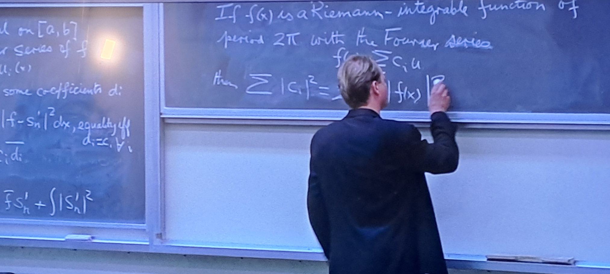
At approximately 00:03:35, Lambeau is finishing a lecture involving Fourier analysis and Parseval’s identity. He asks the class to complete the Parseval material next time and dryly observes that many of them encountered it as undergraduates, so a review will do no harm.

Around 00:03:55, he turns from the lecture to a separate challenge placed on the chalkboard in the hallway (this is where later an “even harder” problem is written down), describing it as an advanced Fourier system. By about 00:04:00, he says that he hopes someone will prove it before the semester ends. A few seconds later he invokes academic fame and recognition—Nobel laureates, Fields Medal winners and other distinguished former names—in a deliberately grand, somewhat sardonic piece of classroom theatre. As you might remember, he is a Fields Medal laureate himself.

The surviving working notes are imperfect dialogue notes, so those lines are paraphrased here rather than polished into invented quotations. What matters for the mathematics is the transition: a Fourier lecture ends, and a challenge is announced. Later, the hallway board presents its concrete graph-theory tasks.

Lambeau at a chalkboard containing a Fourier-series expansion and a Parseval identity. — Lambeau concludes a lecture involving Fourier analysis and Parseval’s identity.

Fourier first, graph theory second

Two mathematical layers appear close together. The lecture board contains Fourier series and a Parseval-type norm identity. The first hallway challenge, by contrast, shows a four-vertex graph and asks about its adjacency matrix, walks and generating functions.

The first blackboard problem is therefore not itself a Fourier-analysis problem. But the subjects are not strangers. Once a symmetric adjacency matrix is decomposed into eigenvectors, ideas about modes, projections and norm preservation return naturally. That bridge is worth crossing later; it should not be mistaken for a hidden step required to solve the four tasks.

The four tasks on the board

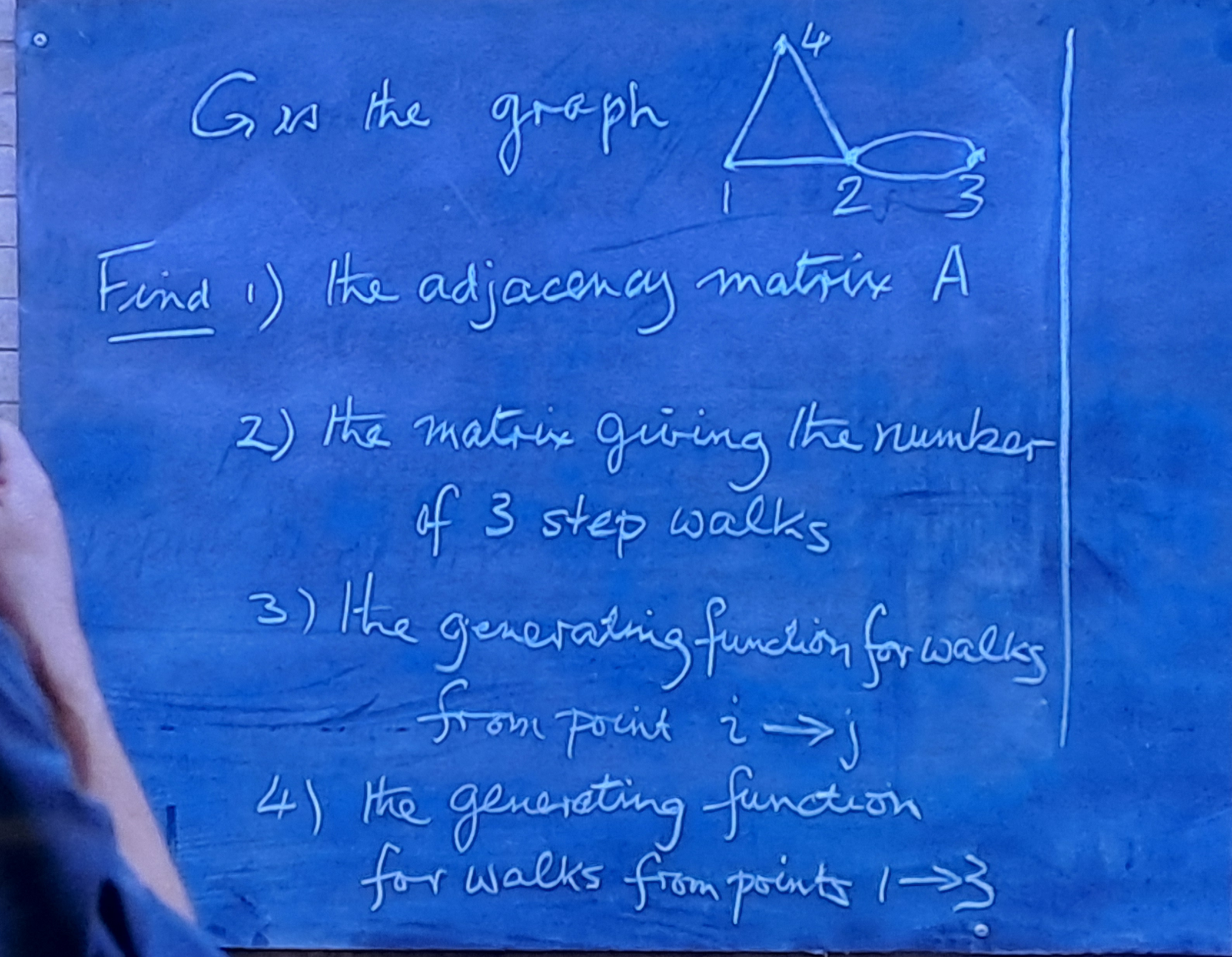
The screenshot shows four connected requests—not merely “find the adjacency matrix.” In clean notation, while preserving the board’s meaning, they are:

Find the adjacency matrix \(A\).
Find the matrix giving the number of three-step walks.
Find the generating function for walks from vertex \(i\) to vertex \(j\).
Find the generating function for walks from vertex \(1\) to vertex \(3\).

The progression is the point. Task 1 encodes the graph. Task 2 discovers what matrix powers count. Task 3 gives a scalar generating function for an arbitrary pair of vertices \(i,j\). Task 4 then specializes that general answer to \(i=1\) and \(j=3\).

The hallway chalkboard showing a four-vertex multigraph and four graph-theory tasks. — The hallway board presents four connected graph-theory tasks.

Task 1: the adjacency matrix

Perhaps a remark first: if you shake your head and say, “I never encountered this in my studies,” that may well be true. Even as a theoretical physicist, I did not meet adjacency matrices in my physics or mathematics courses, but only later in theoretical computer science, in connection with automata theory, Petri nets and related topics. So it would be no surprise if a mathematician, physicist or engineer had never seen this particular use of matrices. Cayley–Hamilton and related matrix identities do appear in finite-dimensional quantum mechanics, but interpreting matrix powers as counts of walks belongs to a different context.

The diagram has four labelled vertices. Vertices 1, 2 and 4 form a triangle; vertices 2 and 3 are joined by two parallel edges. Because a pair of vertices may have more than one edge, this is a multigraph.

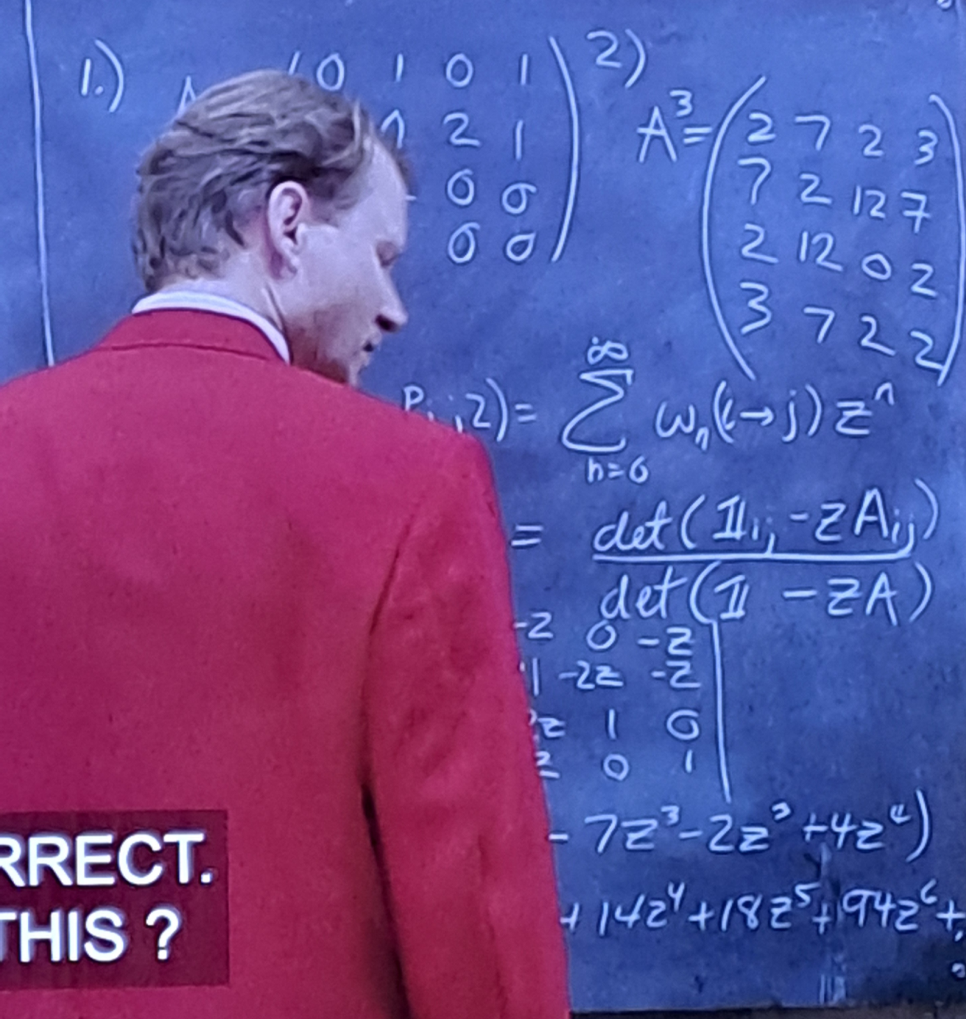
Its adjacency matrix, checked against the graph visible in the screenshot, is

A = \begin{pmatrix} 0 & 1 & 0 & 1 \\ 1 & 0 & 2 & 1 \\ 0 & 2 & 0 & 0 \\ 1 & 1 & 0 & 0 \end{pmatrix}.

Rows and columns correspond to vertices, and \(A_{ij}\) counts edges between vertices \(i\) and \(j\). The graph is undirected, so \(A\) is symmetric. No loops are shown, so every diagonal entry is zero. The entries \(A_{23}=A_{32}=2\) record the two parallel edges between vertices 2 and 3.

Task 2: counting three-step walks

A walk may revisit vertices and edges. The standard adjacency-matrix result is that

(A^n)_{ij}

counts walks of length \(n\) from vertex \(i\) to vertex \(j\), with parallel-edge choices counted separately.

Matrix multiplication explains why. For two steps,

(A^2)_{ij} = \sum_k A_{ik}A_{kj}.

Fix an intermediate vertex \(k\). There are \(A_{ik}\) choices for the first edge and \(A_{kj}\) choices for the second, so their product counts the two-step walks passing through \(k\). Summing over all \(k\) counts every possible intermediate vertex. Repeated multiplication appends further steps, giving the result for \(A^n\).

For this graph, direct multiplication gives

A^2 = \begin{pmatrix} 2 & 1 & 2 & 1 \\ 1 & 6 & 0 & 1 \\ 2 & 0 & 4 & 2 \\ 1 & 1 & 2 & 2 \end{pmatrix},

and then

A^3 = \begin{pmatrix} 2 & 7 & 2 & 3 \\ 7 & 2 & 12 & 7 \\ 2 & 12 & 0 & 2 \\ 3 & 7 & 2 & 2 \end{pmatrix}.

Thus \((A^3)_{13}=2\): exactly two three-step walks run from vertex 1 to vertex 3. They have the vertex sequence \(1\to4\to2\to3\); the final move can use either of the two parallel edges from 2 to 3.

The 12 in \((A^3)_{23}\) is larger but less transparent at a glance. The entry \((1,3)\) makes the multigraph bookkeeping especially easy to see, which is why it is a useful example before Task 4 asks for that same pair of vertices.

Tasks 3 and 4: generating functions

Rather than treating every length separately, introduce a variable \(t\) and collect all powers of \(A\) into

G(t) = I+tA+t^2A^2+t^3A^3+\cdots.

This power series may look familiar. If you’ve taken a first course in Linear Algebra, you might already be thinking of the Cayley–Hamilton theorem. Exactly—that is where the story continues. Later! But for now:

The coefficient of \(t^n\) in the \((i,j)\) entry is \((A^n)_{ij}\), the number of length-\(n\) walks from \(i\) to \(j\). In other words,

g_{ij}(t) = \sum_{n=0}^{\infty} (A^n)_{ij}t^n.

At first, \(t\) is a formal bookkeeping variable. Its powers keep different walk lengths separate. At \(t=1\), however, we would add the numbers of walks of all lengths. Because the graph contains cycles, walks exist for arbitrarily large lengths, so infinitely many terms are at least \(1\). Comparison with \(1+1+1+\cdots\) already shows that the series diverges.

The usual geometric-series cancellation works for matrices:

\begin{aligned} (I-tA) \left( I+tA+t^2A^2+\cdots \right) &= I+tA+t^2A^2+\cdots\\ &\quad{}-tA-t^2A^2-t^3A^3-\cdots\\ &=I. \end{aligned}

Consequently, as a formal power series—and also analytically whenever \(t\) is sufficiently small—

G(t)=(I-tA)^{-1}.

This matrix is a compact way to collect all pairs at once, but Task 3 asks for a scalar function. For fixed vertices \(i\) and \(j\), its answer is the \((i,j)\) entry

\boxed{ g_{ij}(t) = \sum_{n=0}^{\infty}(A^n)_{ij}t^n = e_i^{\mathsf T}(I-tA)^{-1}e_j = \left[(I-tA)^{-1}\right]_{ij} = \frac{C_{ji}(I-tA)}{\det(I-tA)} }.

Here \(e_i\) and \(e_j\) are the corresponding standard basis vectors, so the displayed expression is scalar-valued. Task 4 is the special case \(i=1\), \(j=3\):

g_{13}(t) = \left[(I-tA)^{-1}\right]_{13}.

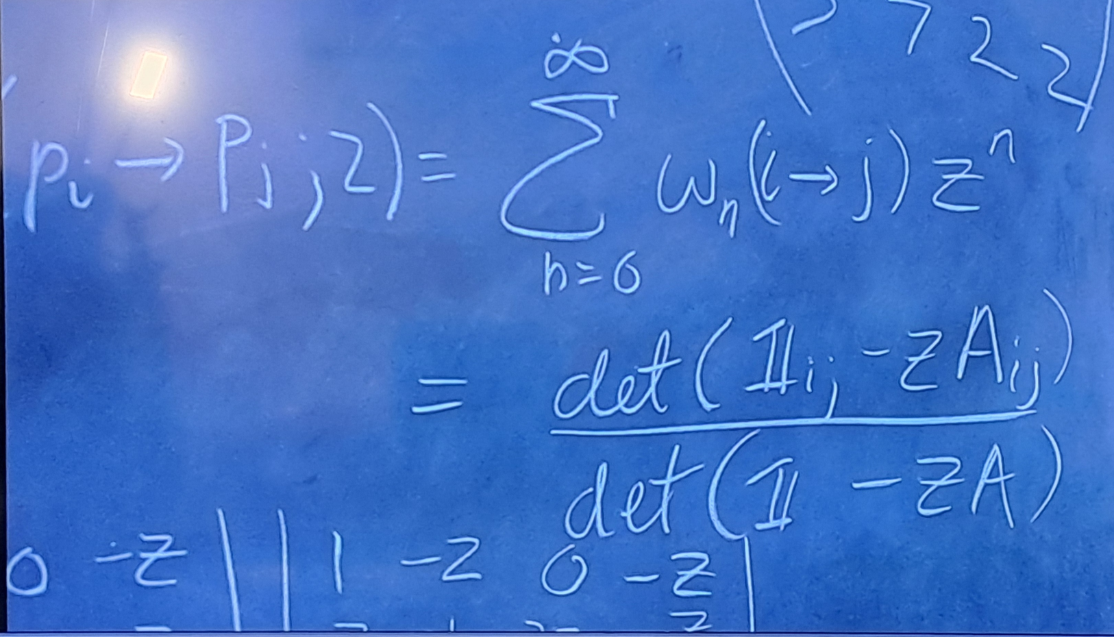
The visible solution board uses the determinant/cofactor route to entries of an inverse. For any invertible matrix \(M\),

(M^{-1})_{ij} = \frac{C_{ji}(M)}{\det(M)},

where the reversed indices are important: \(C_{ji}\) is the cofactor in row \(j\), column \(i\). Applying this to \(M=I-tA\), an independent calculation gives

C_{31}(I-tA)=2t^2+2t^3 \] \[ \det(I-tA)=1-7t^2-2t^3+4t^4.

Therefore the requested scalar generating function is

g_{13}(t) = \frac{2t^2+2t^3} {1-7t^2-2t^3+4t^4}

Both numerator and denominator contain the factor \(1+t\):

2t^2+2t^3=2t^2(1+t), \qquad 1-7t^2-2t^3+4t^4 =(1+t)(1-t-6t^2+4t^3).

After cancelling it, the same generating function has the simpler form

\boxed{ g_{13}(t) = \frac{2t^2}{1-t-6t^2+4t^3} }.

Now perform formal power-series division. Writing

g_{13}(t)=\sum_{n=0}^{\infty}a_nt^n

and comparing coefficients in

(1-t-6t^2+4t^3)g_{13}(t)=2t^2

gives \(a_0=a_1=0\), \(a_2=2\), and, for \(n\geq 3\),

a_n=a_{n-1}+6a_{n-2}-4a_{n-3}.

The division therefore begins

\boxed{ g_{13}(t) = 2t^2+2t^3+14t^4+18t^5+94t^6+\cdots }.

This is the line visible on the solution board. Its coefficients tell the walk-counting story directly: there are no walks of lengths \(0\) or \(1\) from vertex 1 to vertex 3, then \(2\) of length \(2\), \(2\) of length \(3\), \(14\) of length \(4\), \(18\) of length \(5\), and \(94\) of length \(6\).

Detail of the solution board showing walk-count notation and a determinant expression. — The solution uses walk-count notation and the determinant/cofactor formula for an inverse-matrix entry.

Detail of the solution board showing the adjacency matrix, its third power and a generating function. — The adjacency matrix, its third power and the generating-function calculation appear together on the later board.

Why the infinite series has finite structure

The generating function looks infinite:

G(t)=I+tA+t^2A^2+\cdots.

But the powers appearing in it are far less independent than this notation suggests. The reason is the Cayley–Hamilton theorem which may ring a bell (Linear Algebra I): every square matrix satisfies its own characteristic polynomial.

p(\lambda)=\det(\lambda I-A),

then

\[ p(A)=0. \]

For a general \(4\times4\) matrix, write

p(\lambda) = \lambda^4+c_3\lambda^3+c_2\lambda^2+c_1\lambda+c_0.

Cayley–Hamilton gives

\[ A^4+c_3A^3+c_2A^2+c_1A+c_0I=0. \]

Thus \(A^4\) is a linear combination of \(I,A,A^2,A^3\). Multiplying the same identity by \(A\), and then by further powers of \(A\), reduces every higher power \(A^5,A^6,\ldots\) to a combination of those same four matrices. The generating series has infinitely many coefficients, but the matrix algebra needed to express them is finite-dimensional.

For the adjacency matrix in this article, direct calculation gives

p(\lambda) = \lambda^4-7\lambda^2-2\lambda+4.

Consequently,

\[ A^4-7A^2-2A+4I=0, \]

or, equivalently,

\[ A^4=7A^2+2A-4I. \]

That identity already determines all subsequent powers recursively. It is also closely tied to the denominator found above, because

\det(I-tA) = t^4p\!\left(\frac{1}{t}\right) = 1-7t^2-2t^3+4t^4.

The adjugate formula makes the rational form of the generating function explicit:

(I-tA)^{-1} = \frac{\operatorname{adj}(I-tA)} {\det(I-tA)}.

Every entry \(g_{ij}(t)\) is therefore a rational function. Its numerator comes from the corresponding cofactor, while \(\det(I-tA)\)—the characteristic polynomial with the reciprocal substitution above—provides a common denominator. An individual fraction may simplify if numerator and denominator share a factor, but the common algebraic source is the same.

This gives three views of one structure. Cayley–Hamilton supplies a recurrence for matrix powers; the characteristic polynomial supplies its coefficients; and the generating function packages the resulting sequence into rational functions. The eigenvalue decomposition supplies a fourth view.

Why projections and eigenmodes become interesting

The four tasks are complete at this point. Still, the same finite structure offers a natural route into ideas that connect back to the lecture. Because \(A\) is real and symmetric, it admits an orthonormal eigenbasis:

A=Q\Lambda Q^{\mathsf T}.

The columns \(q_k\) of \(Q\) are orthonormal eigenvectors and the diagonal entries \(\lambda_k\) of \(\Lambda\) are the corresponding eigenvalues. Powers and the generating function then become

A^n = Q\Lambda^nQ^{\mathsf T}, \qquad (I-tA)^{-1} = Q(I-t\Lambda)^{-1}Q^{\mathsf T}.

This is useful because powers of a matrix have become powers of scalar eigenvalues. The eigenvalues are precisely the roots of the characteristic polynomial, so this decomposition, Cayley–Hamilton and the rational generating function are different manifestations of the same underlying algebra. Written in terms of rank-one projections,

A = \sum_k \lambda_k q_kq_k^{\mathsf T}, \] \[ A^n = \sum_k \lambda_k^n q_kq_k^{\mathsf T}, \] \[ (I-tA)^{-1} = \sum_k \frac{1}{1-t\lambda_k} q_kq_k^{\mathsf T}.

Each operator \(q_kq_k^{\mathsf T}\) projects a vector onto one eigenmode of the graph. A signal assigning a number to each vertex can be decomposed into these modes, much as an ordinary function can be decomposed into Fourier modes. This is one entrance to spectral graph theory and graph Fourier analysis.

None of this is required to solve Lambeau’s four tasks. It is a mathematical extension: a way to see why adjacency matrices lead naturally from combinatorial counting to questions about spectra, modes and projections.

The road back to Fourier and Parseval

In ordinary Fourier analysis, a function is expanded in an orthogonal basis. Parseval’s identity says, in essence, that the squared norm of the function equals the sum of the squared magnitudes of its Fourier coefficients.

For the orthonormal graph eigenbasis \(q_1,\ldots,q_4\), a graph signal \(f\) has the analogous expansion

f = \sum_k \langle q_k,f\rangle q_k,

and orthonormality gives

\lVert f\rVert^2 = \sum_k \left| \langle q_k,f\rangle \right|^2.

The first blackboard problem is not a Fourier problem. But once its adjacency matrix is viewed through its eigenvectors, the language of modes, projections and Parseval-like norm preservation returns naturally. This is a modern conceptual connection, not evidence that the filmmakers secretly placed an entire graph-signal-processing course inside the scene.

Is the first problem really that difficult?

The first, four-part problem is mathematically genuine. Its sequence from adjacency matrix to walk counts and generating functions is elegant, compact and well suited to a blackboard. The later spectral viewpoint also opens a door to deeper mathematics without being necessary for the original solution.

The film greatly amplifies the exercise’s research-level difficulty. That exaggeration serves the story, but it does not make the board meaningless or badly constructed. A fairer description is that it is a strong connected exercise in graph theory and linear algebra, presented with the dramatic reputation of something much larger. From this point on, the film becomes quite dramatic. A student excitedly reports that “someone solved the theorem!” Yet what appears on the blackboard is not a theorem at all but a carefully designed sequence of exercises—written there by Professor Lambeau himself. He then walks to the board and examines the solution with genuine astonishment. For the audience this creates suspense; mathematically, however, it is difficult to imagine a Fields Medal recipient being baffled by the solution to his own exercise at all.

Conclusion

Many viewers remember the scene as a fantasy of effortless genius. Revisited carefully, it can do something gentler and more useful: remind us how a matrix encodes structure, how its powers count processes, and how familiar ideas about bases and projections reappear in an unexpected setting.

The lecture and hallway boards belong to different topics, but they are not sealed off from one another. The path between them runs through symmetric matrices, eigenmodes and orthogonal projection—a path that is richer than the dramatic myth, and interesting without needing the myth at all.